Users:Structural Optimization/Response Functions/Linear Buckling
Contents |
General Description
Short Info
This response function works similar to the EIGENFREQUENCY_KS response function. The difference is that this response function treat buckling load factors in the Kreisselmeier-Steinhauser function. The provided analysis has to be a linear buckling analysis. By minimizing the Kreisselmeier-Steinhauser function the buckling load factors will be increased.
For this response function the following Kreisselmeier-Steinhauser function is implemented:
- ψ = 1/ρ * ln ∑i e-ρ*λi
with the scaling parameter ρ and the i-th eigenvalue λi of the linear buckling problem
- (Kel - λ*Kgeo) φ = 0.
Input Parameters
| Block headline | ||
| Parameter | Values, Default(*) | Description |
|---|---|---|
| OPT-RESPONSE_FCT | int : LIN_BUCKLING_KS | Function ID and type mechanical problem. |
| Common compulsory parameters | ||
| ETA | real | Finite difference disturbance for sensitivity analysis |
| GRAD | DIRECT, ADJOINT | Method of gradient computation |
| SA | GLOBAL_FD, SEMI_ANALYTIC, EXACT_SEMI_ANALYTIC, ANALYTIC | Method of derivative computations inside sensitivity analysis |
| FDA | FOREWARD, CENTRAL, BACKWARD | Method of finite difference approximation (if neccessary for the chosen sensitivity analysis method) |
| DESVAR | OPT-VAR vector of integers | Design variables that are considered in the sensitivity analysis of this response function |
| Common optional parameters | ||
| WEIGHT | real, 1.0* | The weighting factor for this response function in multi-objective optimization |
| ANALYSIS | PC-ANALYSIS int | ID of the underlying analysis |
| Specific parameters | ||
| RHO | float | Rho parameter of Kreisselmeier-Steinhauser function. Refer to the page Users:Structural Optimization/Response Functions/Eigenfrequency for more information. |
| Common Compulsory Parameters for Constraints | ||
| Parameter | Values, Default(*) | Description |
| REL_LIMIT | real | Relative limit for constraint, depending on the actual value. |
| ABS_LIMIT | real | Absolute limit for constraint. Only one limit can be defined for a constraint. |
| CONSTRAINT_TYPE | INEQUALITY_LT, INEQUALITY_GT, EQUALITY | Type of constraint |
| Common Optional Parameters for Constraints | ||
| REL_TOLERANCE | real, 0* | Upper relative limit until which an inactive constraint is concidered as an active one |
| LAMBDA_ABS_MAX | real, 1/cepsilon* | Upper limit for lagrangian multiplier |
Example of a Complete Input Block
OPT-RESPONSE_FCT 1 : LIN_BUCKLING_KS

  ! -- basic stuff
  WEIGHT=1.0 ANALYSIS=PC-ANALYSIS 1 ETA=1e-06
  GRAD=ADJOINT SA=SEMI_ANALYTIC FDA=FOREWARD
  DESVAR=OPT-VAR 1,2,3,4,5,6

  ! -- response function dependant parameters
  RHO = 2.0

  ! -- constraint parameters
  ABS_LIMIT = 1-e3
  REL_TOLERANCE = 0.1
  CONSTRAINT_TYPE = INEQUALITY_LT
  LAMBDA_ABS_MAX = 20
Example
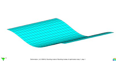
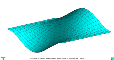
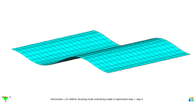
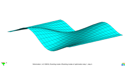
This example considers a flat plate subjected to in-plane compression loading. After reaching a specified load level, the structure starts to buckle. The four smallest buckling modes are presented in the figure below. They result from a linear buckling analysis.
The goal of the optimization problem is to increase the buckling load factors. For this aim the four smallest buckling load factors are formulated in a Kreisselmeier-Steinhauser function. This function serves as objective and is decreased during optimization. All normal nodal coordinates are defined as design variables. This results in 441 design variables. The problem is solved by the Conjugate Gradient Method using a 3-Point Line Search.
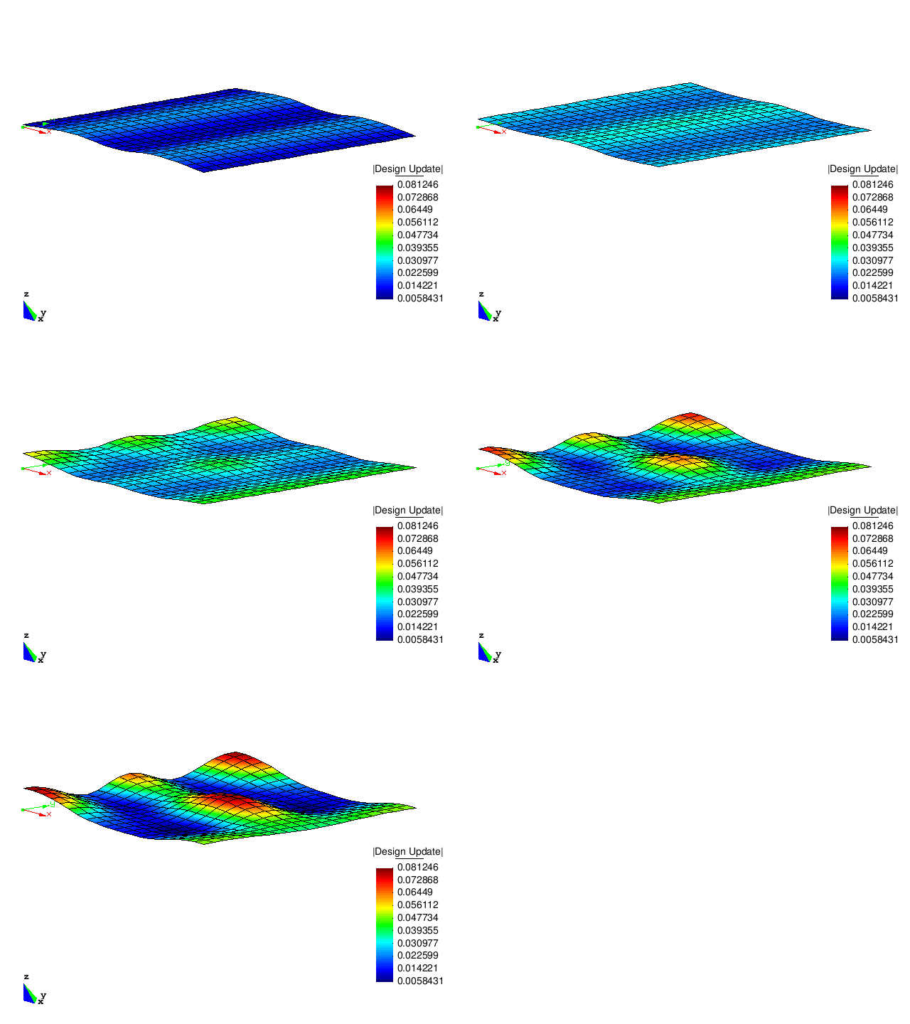
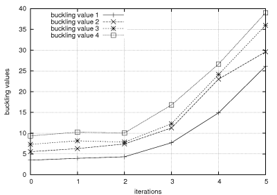
The figure below shows the design updates of the first five optimization steps. It can be clearly observed that the optimized structure has a much higher buckling load than the initial structure.
This is also shown by the curves of the buckling load factors.
| Whos here now: Members 0 Guests 0 Bots & Crawlers 1 |
