Users:Structural Optimization/Response Functions/Eigenfrequency
Contents |
General Description
Short Info
This response function refers to all eigenvalues computed by the eigenvalue analysis. The function itself is a weighted sum of all considered eigenvalues based on the works of Kreisselmeier-Steinhauser [1]. The idea of Kreisseleier-Steinhauser was to formulate a optimization objective function that summarizes several response functions and performs an internal weighting according to the relationship of the function values. The current implementation in Carat++ is a formulation that privileges small eigenvalues whereat the weighting can be controlled via the parameter ρ. The higher ρ is set, the more small values are privileged.
This response function is suitable for the maximization of eigenvalues and the corresponding eigenfrequencies.
Input Parameters
| Block headline | ||
| Parameter | Values, Default(*) | Description |
|---|---|---|
| OPT-RESPONSOSE_FCT | int : EIGENFREQUENCY_KS | Function ID and type of response function |
| Common compulsory parameters | ||
| ETA | real | Finite difference disturbance for sensitivity analysis |
| GRAD | DIRECT, ADJOINT | Method of gradient computation |
| SA | GLOBAL_FD, SEMI_ANALYTIC, EXACT_SEMI_ANALYTIC, ANALYTIC | Method of derivative computations inside sensitivity analysis |
| FDA | FOREWARD, CENTRAL, BACKWARD | Method of finite difference approximation (if neccessary for the chosen sensitivity analysis method) |
| DESVAR | OPT-VAR vector of integers | Design variables that are considered in the sensitivity analysis of this response function |
| Common optional parameters | ||
| WEIGHT | real, 1.0* | The weighting factor for this response function in multi-objective optimization |
| ANALYSIS | PC-ANALYSIS int | ID of the underlying analysis |
| Specific parameters | ||
| RHO | real | Kreisselmeier-Steinhauser parameter which controls the weighting. Recommended range: 1 to 100. For more details see Theory and details |
| Common Compulsory Parameters for Constraints | ||
| Parameter | Values, Default(*) | Description |
| REL_LIMIT | real | Relative limit for constraint, depending on the actual value. |
| ABS_LIMIT | real | Absolute limit for constraint. Only one limit can be defined for a constraint. |
| CONSTRAINT_TYPE | INEQUALITY_LT, INEQUALITY_GT, EQUALITY | Type of constraint |
| Common Optional Parameters for Constraints | ||
| REL_TOLERANCE | real, 0* | Upper relative limit until which an inactive constraint is concidered as an active one |
| LAMBDA_ABS_MAX | real, 1/cepsilon* | Upper limit for lagrangian multiplier |
Example of a Complete Input Block
This section presents the input sequence for a Kreisselmeier-Steinhauser constraint.
OPT-RESPONSE_FCT 1 : EIGENFREQUENCY_KS
 WEIGHT=1.0 ANALYSIS=PC-ANALYSIS 1 ETA=1e-06
 GRAD=ADJOINT SA=SEMI_ANALYTIC FDA=FOREWARD
 DESVAR=OPT-VAR 1
! -- response function dependant parameters
 RHO = 1
! -- constraint parameters
 REL_LIMIT = 1.1
 REL_TOLERANCE = 0.1
 CONSTRAINT_TYPE = INEQUALITY_LT
 LAMBDA_ABS_MAX = 20
A complete test example
Model description
The influence of the paramter ρ will be demonstrated at the example of an arch. The following animation shows the geometry and the first 4 eigenmodes of the system.
This system will be optimized twice, once with ρ=1 and one with ρ=100.

Input File
Here the full input file can be downloaded.
Documented Results
The following figures illustrate the developement of the eigenvalues and the final geometry.
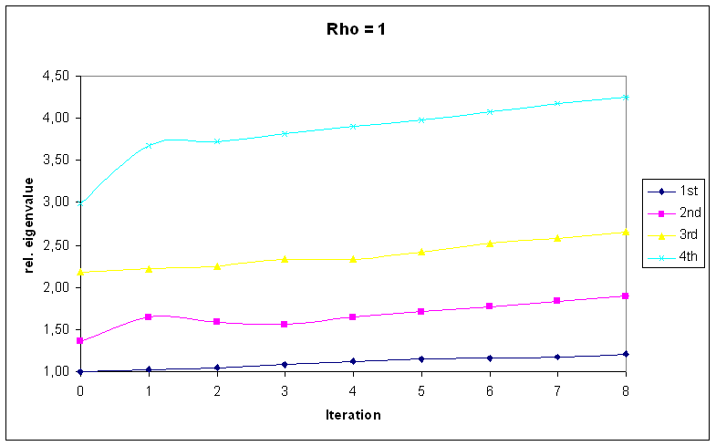
Developement of eigenvalues for Rho=1
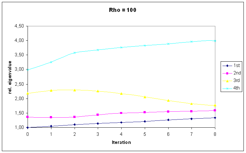
Developement of eigenvalues for Rho=100
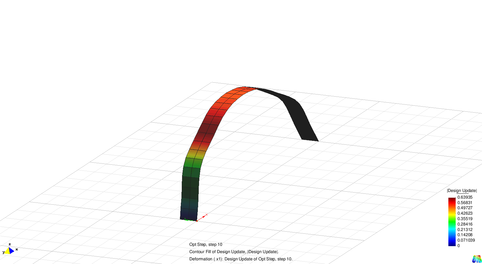
Final geometry (Rho=1)
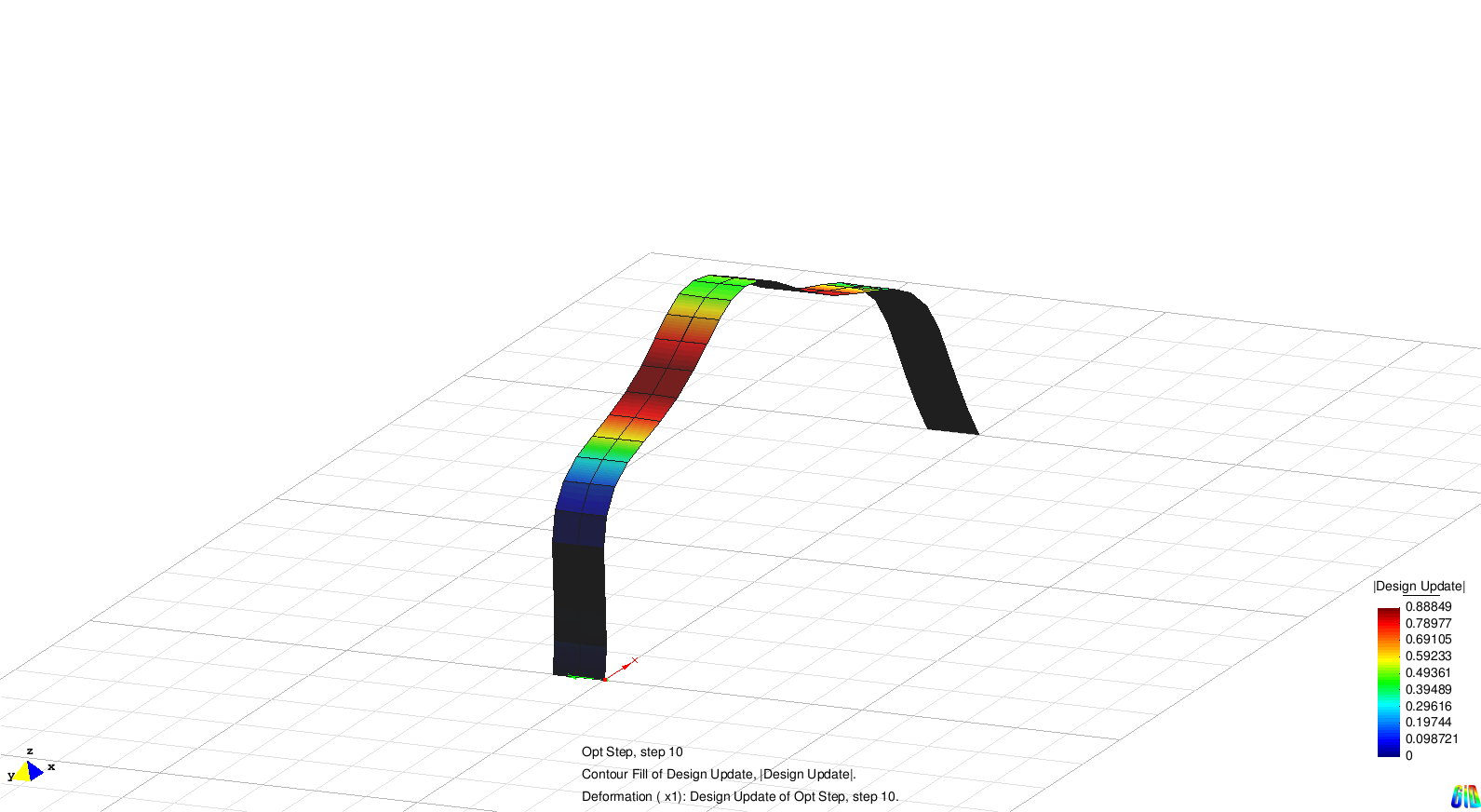
Final geometry (Rho=100)


The first picture shows that for ρ=1 all eigenvalues grow in the process of optimization. Within eight optimization steps they improve by 20 to 40 percent.
In contrast to this, for ρ=100 the first eigenmode is dominant. It increases now 30 percent instead of 20 percent, and at the same time groth of the third and fourth eigenvalue is reduced dramatically. This points out the effect of the control parameter ρ.
Theory and Details
The implementation of the Kreisselmeier-Steinhauser formulation in Carat++ uses the form
 , where λ is a scaled eigenvalue and s is a shifter. Φ will decrease for increasing eigenvalues, and so a minimization of the Kreisselmeier-Steinhauser function leads to a maximization of the eigenvalues.
In order to keep the exponential function from overshooting all limits, a scaling is applied to the eigenvalues. To this purpose for each eigenvalue a scaling factor is computed that way that the initial eigenvalues (at the beginning of the optimization) are mapped onto the interval [0.1, 0.5]. Additionally the shifter s is introduced in order to evaluate the exponential function in a region where it is more curved, and so to force the weighing influence of the formulation. The shifter is set to 80. So for a value of ρ=1 the lowest eigenvalue will reach a value of exp( -1*0.1 + 80 ) = 5e34, which is numerically still acceptable.
References
- ↑ Kreisselmeier, G., and Steinhauser, R., "Systematic Control Design by Optimizing a Vector Performance Index," International Federation of Active Controls Symposium on Computer-Aided Design of Control Systems, Zurich, Switzerland, August 29-31, 1979
| Whos here now: Members 0 Guests 0 Bots & Crawlers 1 |