Users:General FEM Analysis/Analyses Reference/Buckling
Contents |
General Description
This analysis performs a linear estimation of the buckling load factor. To this purpose the system stiffness K is considered to consist of two parts, the elastic stiffness Kel, which is well known from the field of linear static analysis, and the geometric stiffness part Kgeo which is associated to the current state of stress. The complete stiffness can be determined as K = Kel + Kgeo.
The analysis refers to the load factor γ defined by the user in the input deck. Starting from this load factor a linear dependency of the geometric stiffness with respect to the load augmentation factor λ is assumed, and so the critical load augmentation factor where buckling occurs can be estimated by demanding singularity of the complete stiffness (linearized w.r.t. λ):
As the linear dependency of Kgeo w.r.t. λ is a simplifying assumption, the estimated total load carrying factor γ·λ is the more exact the closer λ is to 1. Be aware that in general it is over-estimating the buckling load!
Defining the eigen problem
The equation shown above leads to the solution of an eigen problem similar to the one known from eigenfrequency analysis. The only difference is that instead of det(K-λ·M)=0 we have to solve det(Kel+λ·Kgeo)=0, and so the corresponding eigen problem reads

Input Parameters
Parameter Description
| Compulsory Parameters | ||
| Parameter | Values, Default(*) | Description |
|---|---|---|
| EIGEN_SOLVER | PC-SOLVER int | Linking to an eigen solver |
| LINEAR_SOLVER | PC-SOLVER int | Linking to a linear solver |
| OUTPUT | PC-OUT int | Linking to output objects (specifies the type of output format, e.g. GiD) |
| COMPCASE | LD-COM int | Linking to computation case objects which specify the boundary conditions (loading and supports) |
| DOMAIN | EL-DOMAIN int | Linking to the domain the analysis should work on |
| NUM_ROOT | int | Number of buckling modes and corresponding buckling load factors to determine |
It should be mentioned that the two solvers used within this analysis (linear and eigen solver) have to be compatible with respect to the used sparse matrix format (e.g. both using a Skyline formate or both working on a TRILINOS Csr matrix).
Example of a Complete Input Block
PC-ANALYSIS 1: LINEAR_BUCKLING
EIGEN_SOLVER = PC-SOLVER 1
LINEAR_SOLVER = PC-SOLVER 2
OUTPUT = PC-OUT 1
COMPCASE = LD-COM 1
DOMAIN = EL-DOMAIN 1
NUM_ROOT = 3
Examples
A Full Example: Buckling of a rod
The following example describes a rod buckling problem, where the rod is discretized by (SHELL8)-elements. A built in rod of length 2 is loaded in normal direction by a compressive force of 1. The cross section's bending stiffness is equal to 1750. The buckling load according to Euler's formula computes to

The corresponding input can be found at:
- ..\examples\benchmark_examples\analyses\linbuckl_shell8_I\cbm_shell8_euler_1.dat
The gallery shows the corresponding buckling modes:
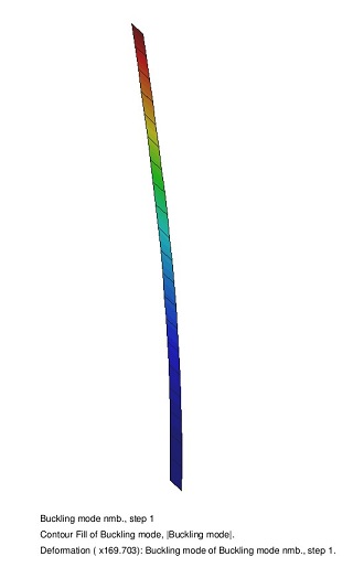
1st buckling mode
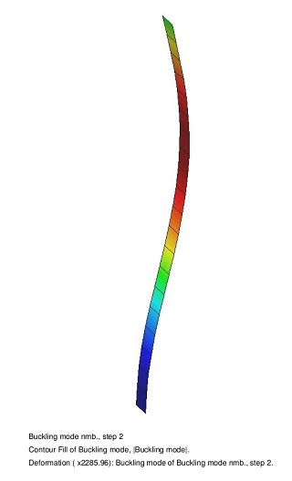
2nd buckling mode
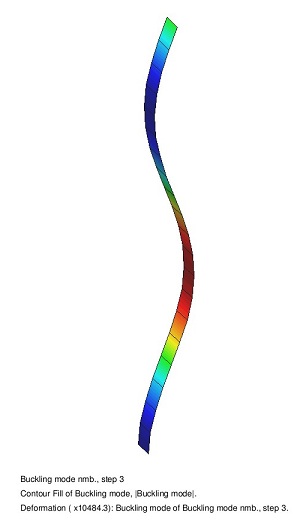
3rd buckling mode
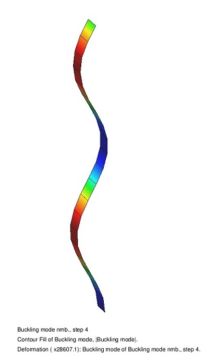
4th buckling mode


The related load factors are computed to:
13:22:12     ###########################################
13:22:12     ### Results of linear buckling analysis ###
13:22:12     ###########################################
13:22:12 Number of buckling modes to compute: 4
13:22:12
13:22:12   Number |   Load Factor    |    Norm of Eigenvector
13:22:12 -------------------------------------------------------
13:22:12     1        1.079266e+03            3.755564e-03
13:22:12     2        9.697325e+03            3.878872e-04
13:22:12     3        2.684653e+04            6.865951e-05
13:22:12     4        5.234735e+04            2.934980e-05
13:22:12 -------------------------------------------------------
13:22:12
13:22:12 Buckling Analysis finished!
So even for a load augmentation factor of more than 1000 the analytical result is met very well.
If the calculation is done with (BEAM1)-elements, the quality of the results is depending on the numbers of buckling modes and the P/Pcrit ratio. For only one buckling mode the applied load should not be less than 5% of the critical load. The minimum applied load approaches the critical load rapidly by increasing the number of buckling modes. In contrast to this there´s no maximum limit.
Benchmark examples
- buckling of an Euler-rod discretized with (SHELL8)-elements : ..\examples\benchmark_examples\analyses\linbuckl_shell8_I\cbm_shell8_euler_1.dat
- buckling of an Euler-rod discretized with (BEAM1)-elements : ..\examples\benchmark_examples\elements\beam1_buckling\cbm_beam1_buckling.dat
- buckling of an Euler-rod discretized with (BEAMCR)-elements : ..\examples\benchmark_examples\elements\BeamCR_LinBuckling\cbm_BeamCR_LinBuckling.dat
| Whos here now: Members 0 Guests 0 Bots & Crawlers 1 |