Users:Structural Optimization/Response Functions/Stress
(→Shell cantilever) |
(→Shell cantilever) |
||
| Line 96: | Line 96: | ||
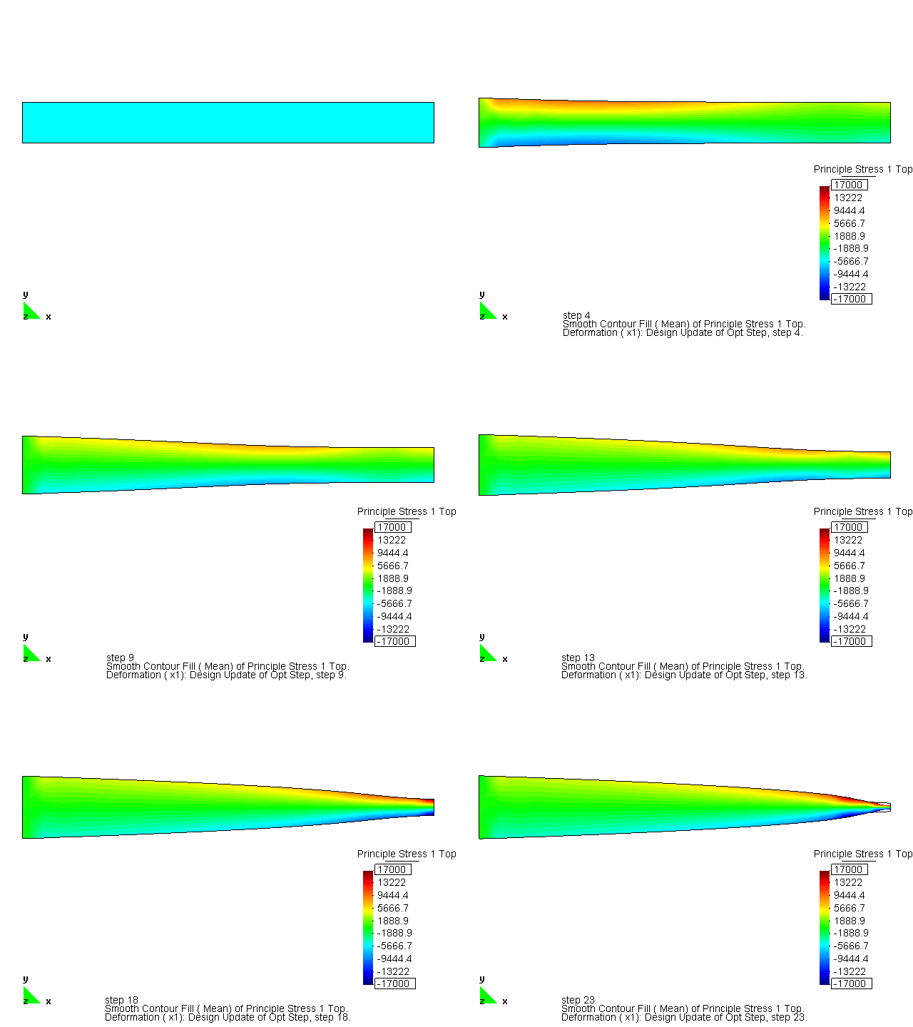
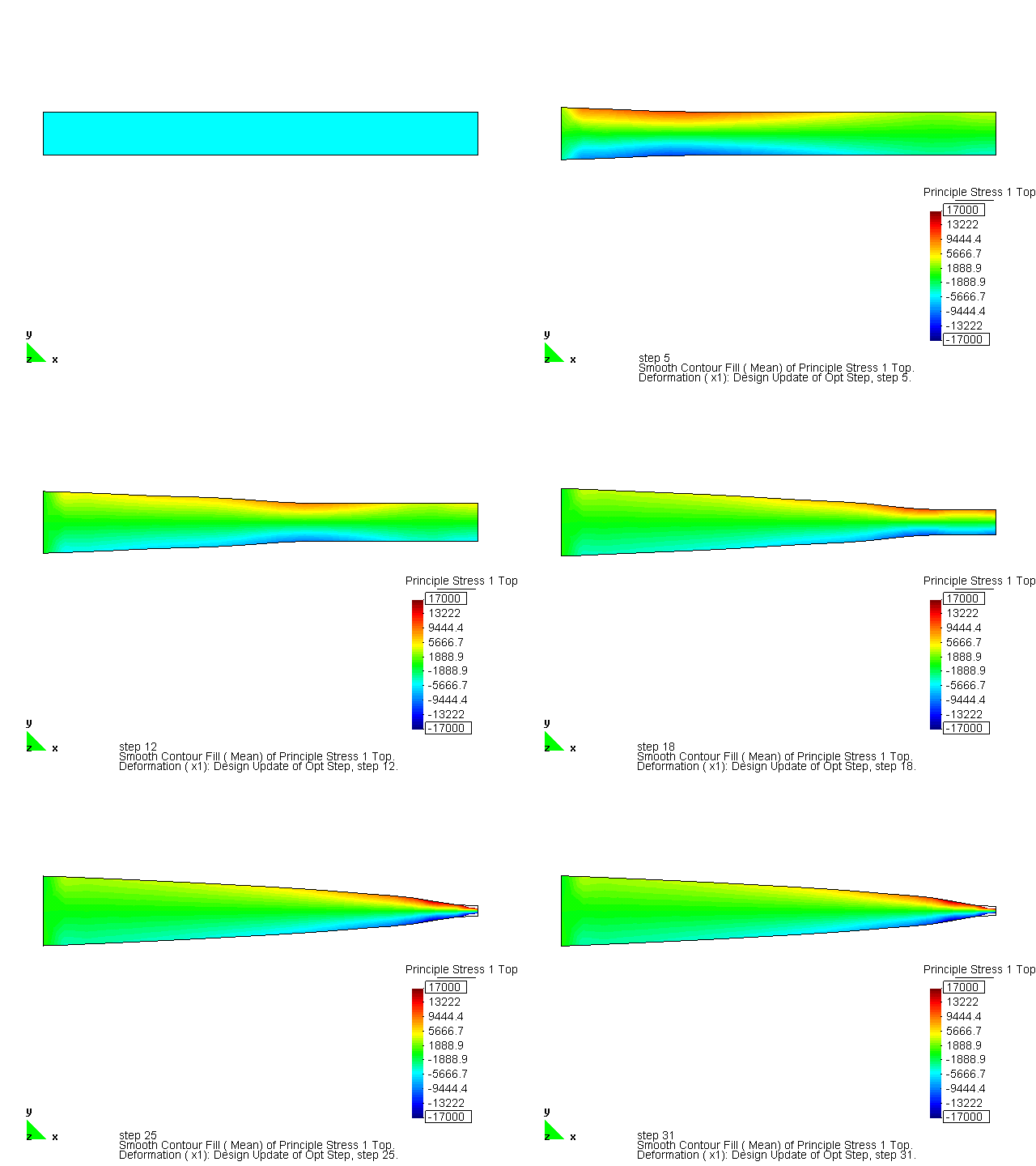
This example shows the optimal shape of a cantilever beam subjected to an end load. The structure is modelled by shell elements. During the optimization, the Kreisselmeier-Steinhauser function is minimized while the structural weight was not allowed to increase more than 5%. To avoid singularity at the free end, a bound constraints the movement of the end nodes. The optimization problem is solved by the Augmented Lagrangian Multiplier method for two values of ρ. Comparing the evolution of the shape, it is clear that the design updates are much more local when using a higher value of ρ. | This example shows the optimal shape of a cantilever beam subjected to an end load. The structure is modelled by shell elements. During the optimization, the Kreisselmeier-Steinhauser function is minimized while the structural weight was not allowed to increase more than 5%. To avoid singularity at the free end, a bound constraints the movement of the end nodes. The optimization problem is solved by the Augmented Lagrangian Multiplier method for two values of ρ. Comparing the evolution of the shape, it is clear that the design updates are much more local when using a higher value of ρ. | ||
| − | + | ||
| − | + | [[ File:Shellcantilever_KS_lowrho.gif |200px | ρ=1]] | |
| − | + | [[ File:Shellcantilever_KS_rho10.gif |200px | ρ=10]] | |
| − | + | ||
Revision as of 15:06, 13 October 2010
Contents |
General Description
Short Info
The Kreisselmeier-Steinhauser function for the stresses is a global measure of stress in a structure. Stress results are generally very local results but using this responce function, an overall stress indicator is obtained. It can be used as an objective to reduce the overall stress in the structure or as a constraint to limit the stress in the structure to a maximum allowed value.
The Kreisselmeier-Steinhauser function for the stresses is formulated by
- KS = 1/ρ log (∑i exp (ρ σi/ σmax ))
with ∑i a summation over all Gausspoints in the domain and σi the stress in the i-th Gausspoint from a linear or nonlinear analysis. σmax is the maximum allowed stress. ρ is a parameter that determines the importance of the largest stresses amongst all σi. The response function requires the ID of a linear static analysis or a nonlinear static analysis specified for parameter 'ANALYSIS'.
(influence of sigma_max) The value of the exponential function becomes infinite very fast, even for reasonable values of the argument. Therefore, the choice of σmax is very important. The best results are obtained if the stresses σi are similar to σmax. If the stresses in the structure are much smaller than the allowed stress, the value of this response function becomes useless. Since it is in that case a summation of all small values, it will be similar for all structures.
(influence of rho)
(so how to choose the values) If this response function is used as an objective function, the value of σmax should be chosen such that it is close to the real stresses in the structure. Additionally, the value for ρ should not be high to use the global stress results. If this response function is used as a constraint function, the value of σmax should be chosen as the real maximum allowed value. Additionally, the value for ρ should be high enough to localize the largest stress.
Input Parameters
| Block headline | ||
| Parameter | Values, Default(*) | Description |
|---|---|---|
| OPT-RESPONSE_FCT | int : STRESS_KS | Function ID and type mechanical problem. |
| Common compulsory parameters | ||
| ETA | real | Finite difference disturbance for sensitivity analysis |
| GRAD | DIRECT, ADJOINT | Method of gradient computation |
| SA | GLOBAL_FD, SEMI_ANALYTIC, EXACT_SEMI_ANALYTIC, ANALYTIC | Method of derivative computations inside sensitivity analysis |
| FDA | FOREWARD, CENTRAL, BACKWARD | Method of finite difference approximation (if neccessary for the chosen sensitivity analysis method) |
| DESVAR | OPT-VAR vector of integers | Design variables that are considered in the sensitivity analysis of this response function |
| Common optional parameters | ||
| WEIGHT | real, 1.0* | The weighting factor for this response function in multi-objective optimization |
| ANALYSIS | PC-ANALYSIS int | ID of the underlying analysis |
| Specific parameters | ||
| ELEMENTS | El-SET or PART | Determines the elements of which the stress is taken into account |
| STRESS_TYPE | VMISES_TOP, VMISES_BOTTOM, VMISES, PRINCIPLE_1_TOP, PRINCIPLE_1_BOTTOM, PRINCIPLE_1 | Determines which stress type is taken into account |
| RHO | real | Parameter that determines how local the effect of this response function is |
| STRESS_LIMIT | integer | Maximum value for the real value of the stress (cannot be combined with ABS_STRESS_LIMIT) |
| ABS_STRESS_LIMIT | integer | Maximum value for the absolute value of the stress (cannot be combined with STRESS_LIMIT) |
| Common Compulsory Parameters for Constraints | ||
| Parameter | Values, Default(*) | Description |
| REL_LIMIT | real | Relative limit for constraint, depending on the actual value. |
| ABS_LIMIT | real | Absolute limit for constraint. Only one limit can be defined for a constraint. |
| CONSTRAINT_TYPE | INEQUALITY_LT, INEQUALITY_GT, EQUALITY | Type of constraint |
| Common Optional Parameters for Constraints | ||
| REL_TOLERANCE | real, 0* | Upper relative limit until which an inactive constraint is concidered as an active one |
| LAMBDA_ABS_MAX | real, 1/cepsilon* | Upper limit for lagrangian multiplier |
Example of a Complete Input Block
OPT-RESPONSE_FCT 1 : STRESS_KS

  ! -- basic stuff
  WEIGHT=1.0 ANALYSIS=PC-ANALYSIS 1 ETA=1e-06
  GRAD=ADJOINT SA=SEMI_ANALYTIC FDA=FOREWARD
  DESVAR=OPT-VAR 1,2,3,4,5,6

  ! -- specific
  ELEMENTS = EL-SET 1
  STRESS_TYPE = PRINCIPLE_1_TOP
  RHO = 10.0
  ABS_STRESS_LIMIT = 200.0E06

  ! -- constraint parameters
  ABS_LIMIT = 1-e3
  REL_TOLERANCE = 0.1
  CONSTRAINT_TYPE = INEQUALITY_LT
  LAMBDA_ABS_MAX = 20
Examples
Shell cantilever
This example shows the optimal shape of a cantilever beam subjected to an end load. The structure is modelled by shell elements. During the optimization, the Kreisselmeier-Steinhauser function is minimized while the structural weight was not allowed to increase more than 5%. To avoid singularity at the free end, a bound constraints the movement of the end nodes. The optimization problem is solved by the Augmented Lagrangian Multiplier method for two values of ρ. Comparing the evolution of the shape, it is clear that the design updates are much more local when using a higher value of ρ.
| Whos here now: Members 0 Guests 0 Bots & Crawlers 1 |

