Users:General FEM Analysis/BCs Reference
Contents |
Load case
A load case object collects all boundary conditions, Dirichlet and Neumann constraints, which define the current problem. A load case block is linked directly into an analysis object. Each Neumann block is separately weighted by a factor FAC.
The example below shows a load case including a nodal load block, one element load and one set of Dirichlet conditions.
LD-COM 1
 TYPE = LD-NODE 1    FAC=1.0
 TYPE = LD-ELEM 1    FAC=1.0
 TYPE = BC-DIRICHLET 1
Dirichlet Boundary Conditions
Dirichlet conditions can be divided into three groups: single point constraints (SPC) which refer to one point only and multiple point constraints (MPC) that perform a kind of coupling by applying the same Dirichlet object to several points. The RBE condition bulids up the last group, which defines a coupling in between several points, but each point computes its own displacement according to a certain formula.
SPC-ZERO
The SPC-ZERO condition is the most frequently used Dirichlet condition. It prescribe zero displacement to certain nodes of a point. To this purpose it is necessary to list the influenced nodes and the related fixed DOFs inside the Dirichlet block.
BC-DIRICHLET 1 : SPC-ZERO
  NODE 1    DISP_X  DISP_Y   DISP_Z     ! fix all translatoric DOFs for node 1
  NODE 2    DISP_X                      ! only fix the translation in x-direction for node 2
  NODE 3    DIR_DIFF_SHELL8_X           ! the director related degrees of freedom of the SHELL8 can be equipped with Neumann BCs, too
SPC-NONZERO
The SPC-NONZERO condition allows to prescribe a nodal displacement unequal zero (eg. settlement of a support). The handling is quite similar to the SPC-ZERO, but each considered degree of freedom needs to be assigned a value.
REMARK: This BC is currently only available for geometrical non-linear computations.
As an example we regard a cantilever with a prescribed tip displacement of 1.
BC-DIRICHLET 2: SPC-NONZERO NODE 721 DISP_Z = 1 NODE 722 DISP_Z = 1 NODE 723 DISP_Z = 1 |

|
SPC-DIRECTION
This condition allows to limit translatoric movements of a point within a plane or a line. To this purpose a plane is defined by the parameter DIRECTION_1 naming the plane normal. If a second plane is defined by specifying DIRECTION_2 the point is only allowed to move an the intersection line of the two planes.
This will be shown on a short example. A truss element defined by nodes 1 and 2 is located along the global x-axis. Point 1 is fixed in all three directions and at node 2 a tensile force is applied. As an additional constraint, node 2 is forced to move along the line defined by the vector (1,1,1). To this purpose, two Dirichlet blocks have to be defined. The fist one is a SPC-ZERO block fixing node 1 (not listed here), and the second one limiting node 2 to a one dimensional movement using a SPC-DIRECTION constraint:
BC-DIRICHLET 2: SPC-DIRECTION
  DOFS=DISP_X DISP_Y DISP_Z    NODES=2   DIRECTION_1 = -1,0,1    DIRECTION_2 = 0,1,-1
where the vector (1,1,1) is defined indirectly by two directions being normal to it.
The picture below shows the result with the tip displacement visualized by an arrow.

If the same directions have to be applied to several nodes this can either be done by listing the node vector inside the BC-block or by using node sets:
  DOFS=DISP_X DISP_Y DISP_Z    NODES=2,3,4          DIRECTION_1 = -1,0,1    DIRECTION_2 = 0,1,-1
  DOFS=DISP_X DISP_Y DISP_Z    NODE-SET= ND-SET 5   DIRECTION_1 = -1,0,1    DIRECTION_2 = 0,1,-1
Another method of prescribing a direction is the usage of the nodal director. It either can be defined in reference or in actual configuration:
  DOFS=DISP_X DISP_Y DISP_Z    NODES=1          DIRECTION = NODE_DIR_REF
  DOFS=DISP_X DISP_Y DISP_Z    NODES=2          DIRECTION = NODE_DIR_ACT
MPC-COUPLING
An instance of MPC-COUPLING allows degrees of freedom of different nodes to share the same equation number, so they assemble to the same entries inside global matrices and vectors and return identical results. Of course only degrees of freedom of the same type can be coupled.
An application for a coupling instance might be the modelling of an hinge. Two nodes are defined at the same coordinates and coupled via their translatoric DOFs:
NODE 1   X 0  Y 0  Z 0
NODE 2   X 0  Y 0  Z 0
   .....
BC-DIRICHLET 1 : MPC-COUPLING
  DOFS = DISP_X  DISP_Y  DISP_Z    NODES=1, 2
RBE
If a rigid body element has to be defined, the Dirichlet condition RBE can be used. To this purpose a master node has to be defined which controls the motion of the hole rigid body. All other nodes compute their displacements depending on the translations and rotations of the master node.
The section below shows the definition of a 10-noded rigid body.
BC-DIRICHLET 1 : RBE
  MASTERNODE = NODE 1
  DOFS = DISP_X  DISP_Y  DISP_Z   NODES = 2,3,4,5,6,7,8,9,10
As an example we consider a cantilever loaded by a tip moment. Within the first computation we did not define a rigid body element and so the cantilever curves along its complete length (the red line deviates from the centre line of the green part). For the second run we defined the green part to be a rigid body. As a result, this part does not curve at all (the red line is identical with the centre line).
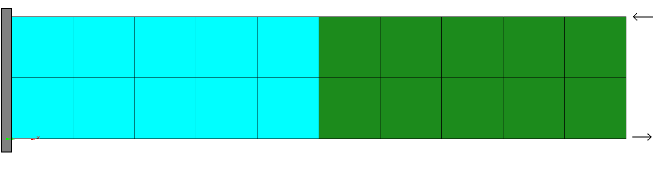
initial geometry
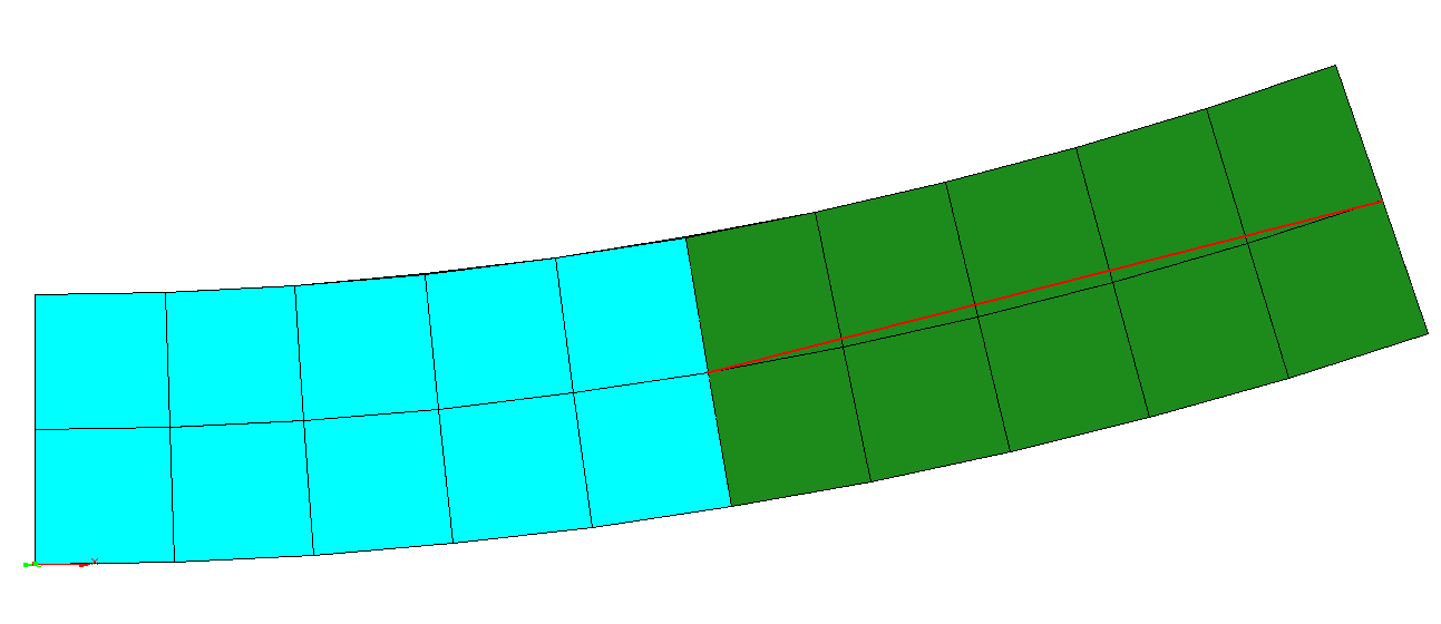
result without RBE
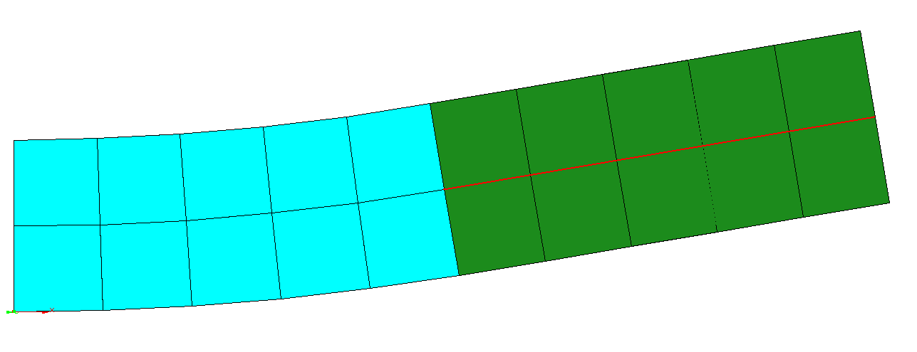
result with RBE defined


Neumann Boundary Conditions
Some general remarks concerning Neumann conditions:
- The parameter LD-CURVE is an optional input. It is only used in dynamic analyses. For non-linear statics the load curve has to be defined in the analysis block.
LD-NODE
A node load is the most simple kind of Neumann boundary condition. A force or a bending moment is directly applied to a finite element node, whereat the load is defined by its direction and its value. The length of the direction defining vector [D1, D2, D3] does not play any role.
LD-NODE 1  TYPE = FORCE    LD-CURVE = LD-CURVE 1
  NODE 1   D1 = 1.0   D2 = 0.0   D3 = 0.0   VAL = 10
  NODE 2   D1 = 0.0   D2 = 0.0   D3 = 1.0   VAL = 20
LD-ELEM
A more complex way of defining Dirichlet conditions is to apply a constraint not to a node but to an element, so the element itsself has to determine its equivalent nodal forces. Depending on the direction and the influenced area one can distinguish between snow load, dead load and pressure load.
PRES
Pressure is an element load acting on an element surface. It is usually acting normal to the element surface, so defining a direction is not necessary. If a different acting direction is desired it can be defined via the direction vector in local element coordinates. The load value is equal to the value entered in the load definition.
LD-ELEM 1 PART=1 LD-CURVE = LD-CURVE 1 TYPE=PRES VAL=10 ! input using default direction D1=0 D2=0 D3=1 ! alternative input for pressure parallel to the element surface acting parallel to the element's 1st local coordinate TYPE=PRES D1=1.0 D2=0.0 D3=0.0 VAL=10 |

|
SNOW
Snow load is also an element surface related load. In contrast to pressure load it is defined by a direction and it is not acting onto the complete element surface but on its projection into the plane normal to the direction of action. The picture below shows snow load acting into z-direction onto an inclined element.
LD-ELEM 1 PART=1 LD-CURVE = LD-CURVE 1 TYPE=SNOW D1 = 0.0 D2 = 0.0 D3 = 1.0 VAL=10 |

|
DEAD
Dead load is acting onto the whole volume of an element. It is computed by multiplying material's density times the load value, which should be equal to gravity's acceleration. Gravity's direction can be defined by the direction vector [D1, D2, D3]. The following input block represents material and load parameters for concrete material and gravity acting in z-direction.
EL-MAT 1 : LIN_ELAST_ISOTROPIC EMOD=3.5e10 ALPHAT=1e-5 DENS=2.5e3 NUE=0.2 LD-ELEM 1 PART=1 LD-CURVE = LD-CURVE 1 TYPE=DEAD D1=0.0 D2=0.0 D3=1.0 VAL=9.81 |

|
TEMPERATURE
(This part is currently under development. Author: Helmut. Date: 08/2010.)
The second kind of volume load is the temperature load object. In contrast to the loads mentioned above it is not defined by elements but by nodes, as the underlying temperature field is defined by nodal values. To this purpose it is possible to define multiple temperature layers at one node, for example top and bottom layer of a shell.
As an example we consider a U-shaped cantilever, where we describe a temperature of +10 over reference temperature at the lower edge and -10 below reference temperature at the top edge.
LD-ELEM 1 TYPE = TEMPERATURE INTERPOLATE_PART = 1 ND-SET = 30 LAYER = 1 VAL = 10 ND-SET = 23 LAYER = 1 VAL = -10 |

|
Although we only prescribed the temprature at the upper and lower edge we receive a temperature filed which is linear over the height. This is due to the fact that we inputed INTERPOLATE_PART = 1 which forces to interpolate the temperature field for all nodes belomging to part 1. If one omited this input flag all nodes offside the defined edges would be assigned reference temperature and so the displacement would differ significantly.
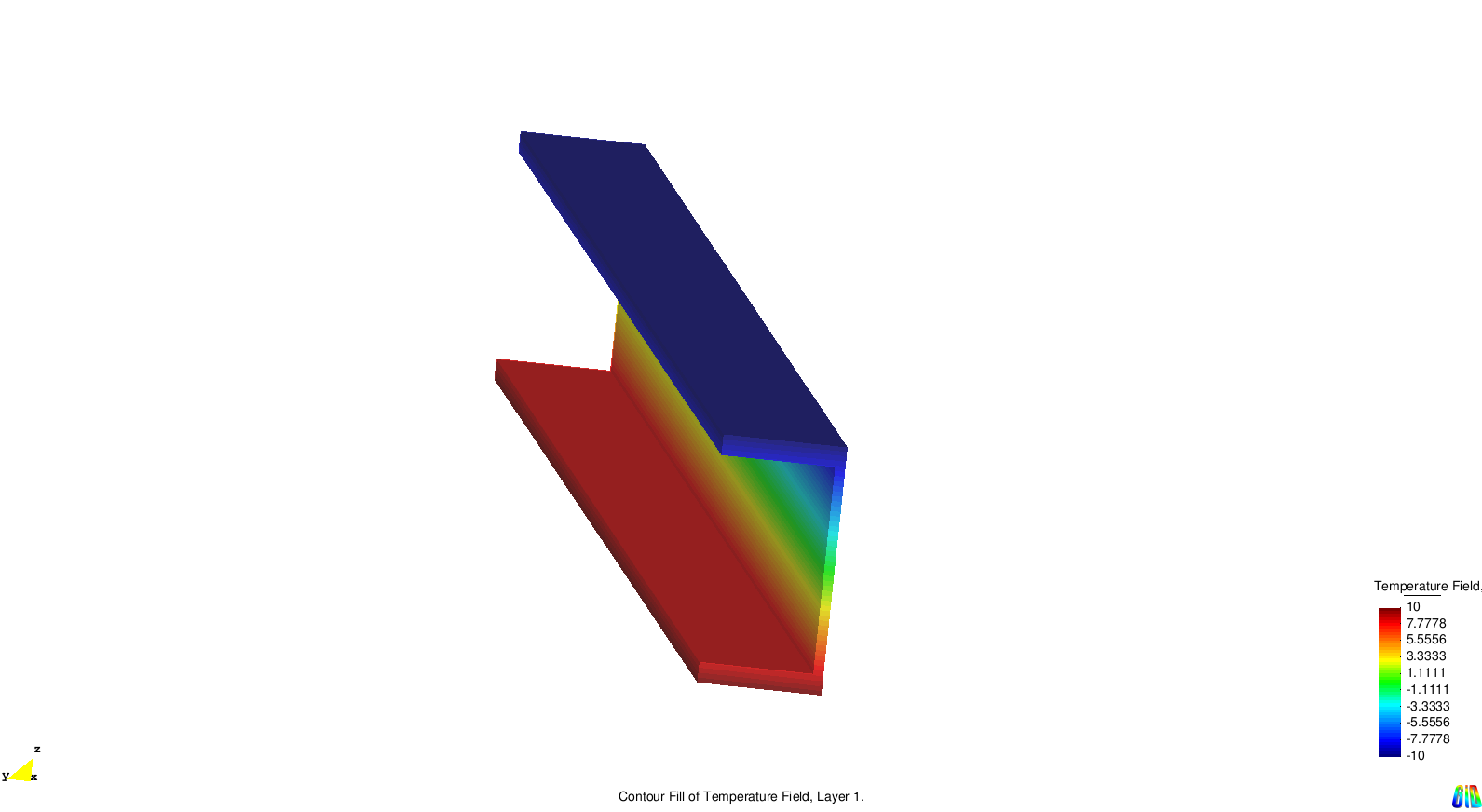
temperature field after inperpolation was applied
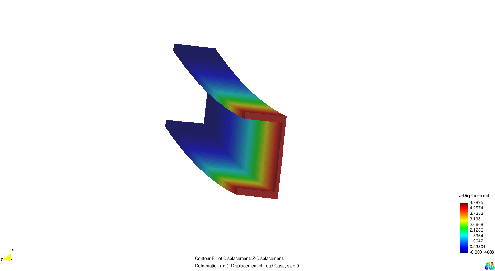
resulting displacement
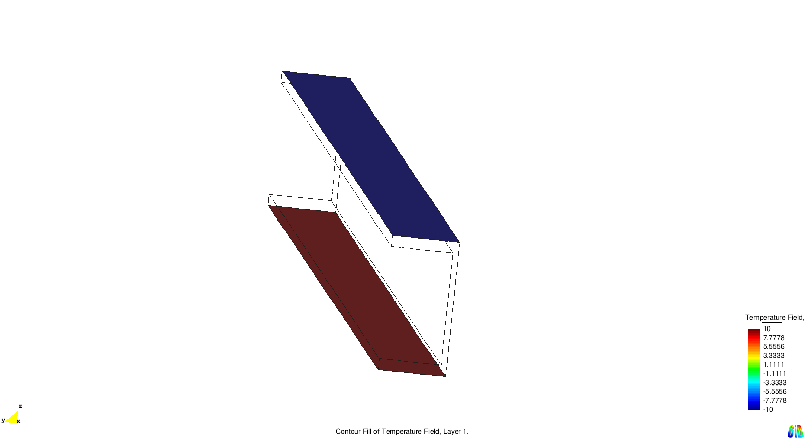
temperature field without inperpolation
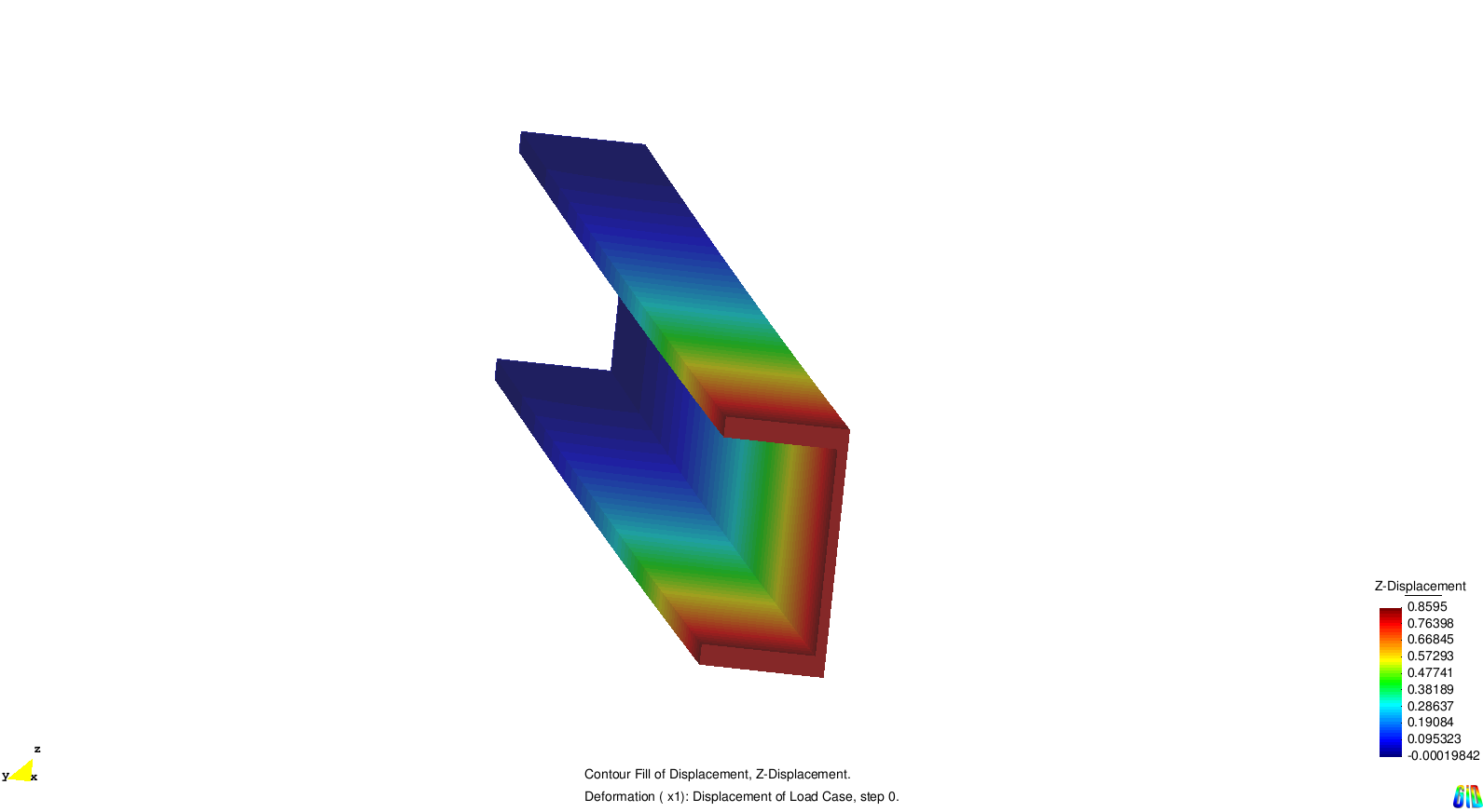
resulting displacement


Load curve
A load curve is used to define time depending load factors for non-linear static analysis or dynamics.
The concept is quite simple: The user specifies a discrete load factor-time-function and values in between are interpolated linearly.
LD-CURVE 1 TYPE=DISCRETE TIME = 0.000 VAL = 0.0000 TIME = 1.000 VAL = 1.0000 TIME = 10.000 VAL = 2.0000 TIME = 12.000 VAL = 0.0000 |
Hints:
|
| Whos here now: Members 0 Guests 0 Bots & Crawlers 1 |