Users:Structural Optimization/Optimization Algorithms/Filtering
Contents |
Motivation
One advantage of finite element based optimization is the huge designspace giving the most possible freedom to the optimization algorithm. Unfortunately this advantage might turn out as a drawback, too. As the design space is very big, the algorithm is enabled to produce short-waved solutions which usually are not intended by the user. For this reason a smoothing has to be applied to the gradient field in order to obtain a minimum wave length inside the design update.
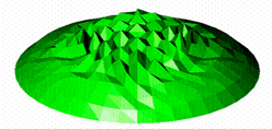
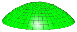
The following pictures show the design update of a circular plate without any filtering, being severely polluted by short waved noise, and a design update after the application of a filter.
|
|
| Design update without filtering | Design update after filter application |
Input
The input of filter functions is separated into two input blocks. The block OPT-FILTER specifies all data that defined the filtering concept. The block OPT-LINKFUNC defines all data related to the specific filter function.
Input parameters
Block OPT-FILTER
| Compulsory Parameters | ||
| Parameter | Values, Default(*) | Description |
|---|---|---|
| OPT-FILTER | int TYPE | ID and filter concept. Actually topological (TYPE = TOPO) and global (TYPE = GLOBAL) filter concepts are available |
| FUNCTIONS = OPT-LINKFUNC 1 | OPT-LINKFUNC int, int, ... | one or more filter functions that should be used |
Two exemplary input blocks
OPT-FILTER 1 : TOPO
  FUNCTIONS = OPT-LINKFUNC 1
!
OPT-FILTER 1 : GLOBAL
  FUNCTIONS = OPT-LINKFUNC 1, 2, 3
Block OPT-LINKFUNC
| Compulsory Parameters | ||
| Parameter | Values, Default(*) | Description |
|---|---|---|
| OPT-LINKFUNC | int TYPE | ID and type of filter function. Actually only circular filter functions are available (TYPE = CIRC) |
| SHAPE | CONST, LIN, QUAD, CUB | function shape; constant, linear, quadratic or cubic |
| RADIUS | real | Radius that defines filter function |
| Optional Parameters | ||
| Parameter | Values, Default(*) | Description |
| MINIMUM_RADIUS | real | Minimum radius for dynamic filter radius (default value = RADIUS) |
| BOUNDARY_RADIUS | real | Radius of boundary blending function (default value = RADIUS) |
| PERFORM_DIRECTION_WEIGHTING | 0*, 1 | Decides if direction weighting is used (1) or not (0) |
| CONCIDER_BLOCK_INTERACTION | 0, 1* | This parameter controls if design varaiables out of other OPT-VAR blocks are concidered for filtering (1) or not (0) |
Exemplary input block
OPT-LINKFUNC 1 : CIRC
 SHAPE=QUAD
 RADIUS=200
 MINIMUM_RADIUS = 50
 BOUNDARY_RADIUS = 80
 PERFORM_DIRECTION_WEIGHTING = 1
 CONCIDER_BLOCK_INTERACTION = 0
Theory
Convolution
The idea of gradient filtering is mathematically based on the theory of convolution integrals.
A mathematical convolution of two functions is defined by [1]
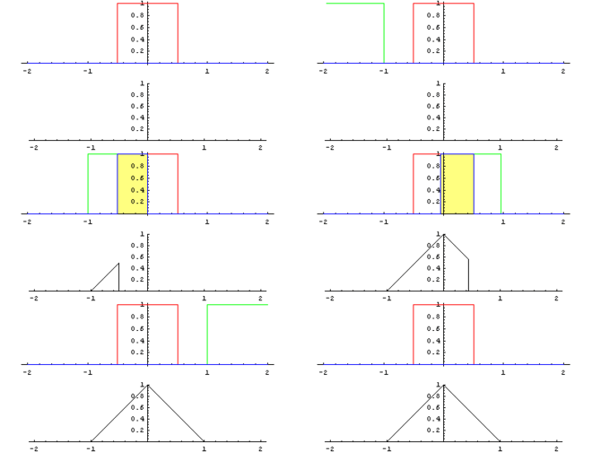
Geometrically a convolution can be interpreded the way that a time dependant function g is weighted by another function f, where the result is computed as the integral of the overlapping interval. The following animation shows the convolution of a constant function with itsself, yielding in a triangular function. [1]
The filter functions in Carat++
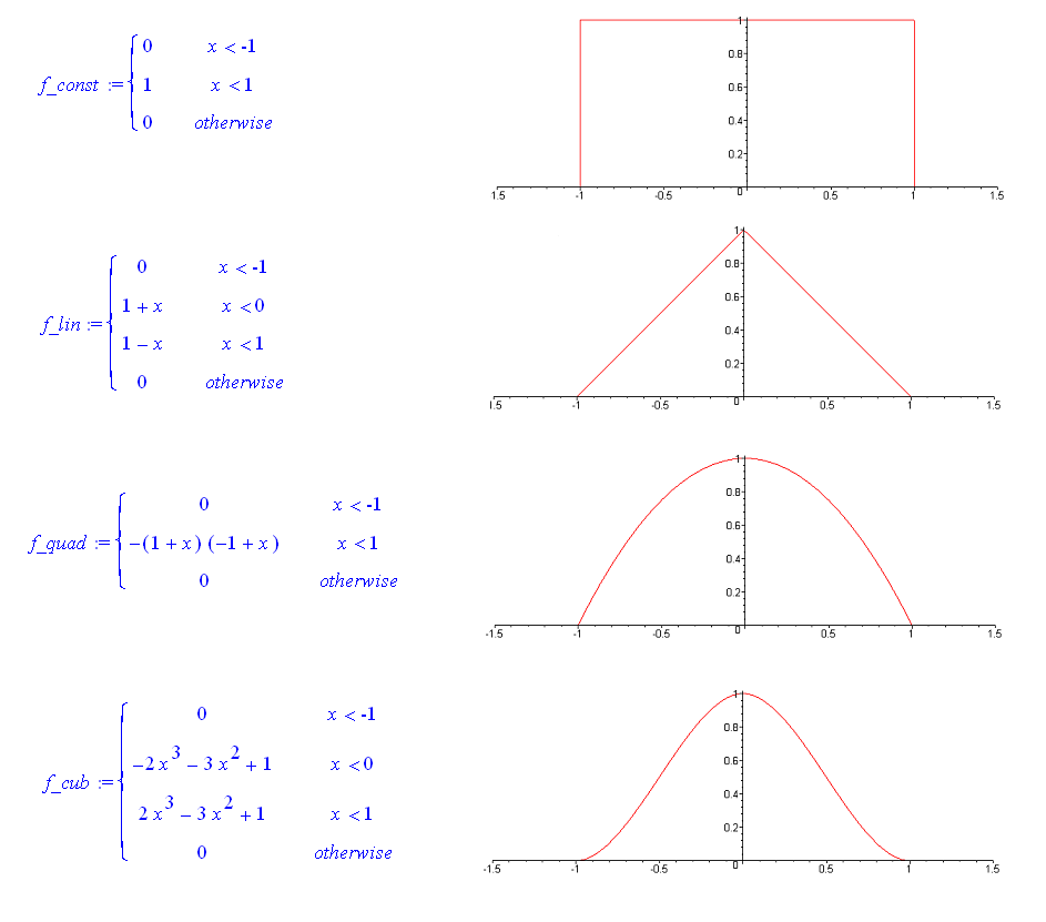
In order to obtain a smooth gradient characteristic, the noisy gradient function is convoluted with a smoothening or filter function. The filter function is defined to be greater than zero inside the filter radius arround the target design variable and equal to zero out of it. The following figure shows the filter functions available in Carat++ which are of constant, linear, quadratic or cubic shape. Note that this figure is just meant to get an impression. The 'real' filter functions are schaled this way that the volume of the body arising by rotating the function arround the y-axis is equal to one depending one the filter radius (which is set to 1 in the figure).
A short example
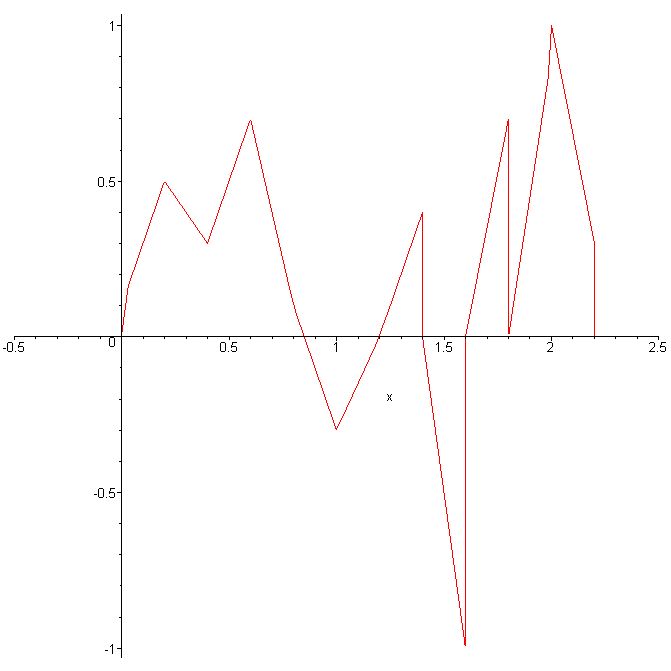
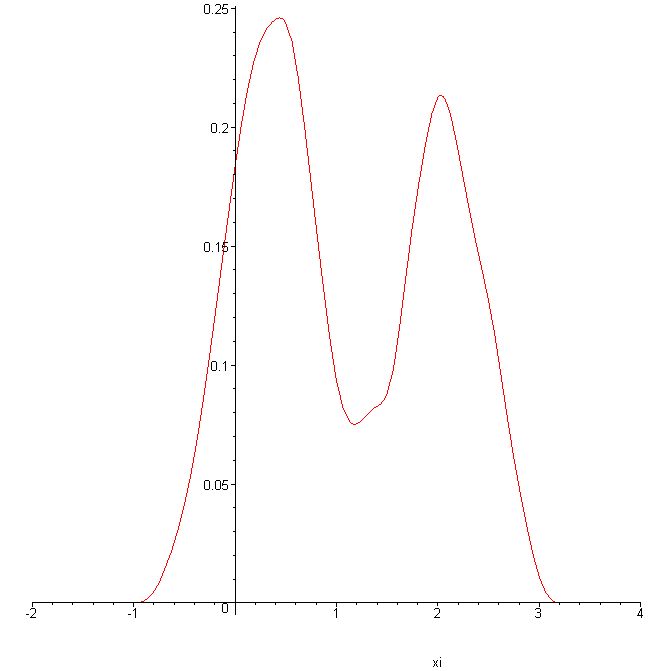
In this paragraph a short example of smoothing by convoluting is shown. To this purpose we define a Co-continous function which is arbitrary in other respects. Then a convolution using the linear and cubic filter function described above is perfomed.
|
|
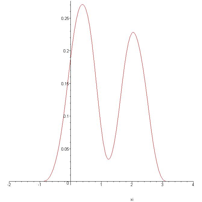
|
| Noisy input function | Result of convolution with linear filter function | Result of convolution with cubic filter function |
This example shows that the smoothing keeps up the general characteristics of the initial function, but extreme values are "cut off" for the sake of smoothness.
Implementation
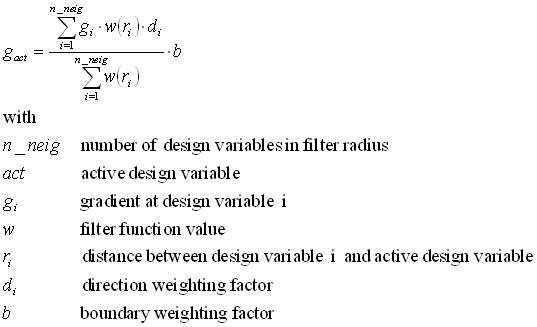
The section above presented the mathematical backgroud of convolution concidering continous functions. As in FE-based optimization the input information for the filtering, the nodal gradients, is a discrete information, the integration within the convolution can be replaced by a summation. So the filtering routine takes the following steps:
- Loop all design variables, define the active design variable
- Determine all design variables that are allocated inside the filter radius arround the active design variable
- Loop all gradient fields (Objecitve(s), constraints)
- Loop all neighboring design variables, determine the filter function's value depending on the distance to the active design variable and compute the gradient of the actual design variable according to the formula:
The parameters b and d are explained in the section Advanced features
Advanced features
Direction weighting
This feature allows to perform an additional weighting with respect to design variable directions. In some applications it is desired that the influence of a design variable onto the filter result decreases if the angle beteen the active design variable and the eighboring design variable increases. To this purpose the direction weighting factor d_i is introduced. It is computed by the scalar product of the active design variable's direction and the directon of the analogous neighboring design variable, but it is not allowed to become negative. So if the nagle in between two design variables exceeds 90 degrees, they do not influense each other within the filtering at all.
If the input parameter PERFORM_DIRECTION_WEIGHTING is set to 0 d_i equals one for all design variables.
Design space boundary weighting
In many applications it appears that a finite element model consists of parts which are defined as design space and other parts that are not allowed to change their geomerty. This feature can be used to generate a smooth transition between this two parts. To this purpose the joint is defined as DESIGN_SPACE_BOUND inside the optimization control block. As a concequence, all gradients withing the BOUNDARY_RADIUS arround the DESIGN_SPACE_BOUND are weighted by an additional boundary smoothing function. This is a 1D quadratic function, being zero at the design space, being one at a distance of BOUNDARY_RADIUS off the bound and showing a horizontal tangent at this point.
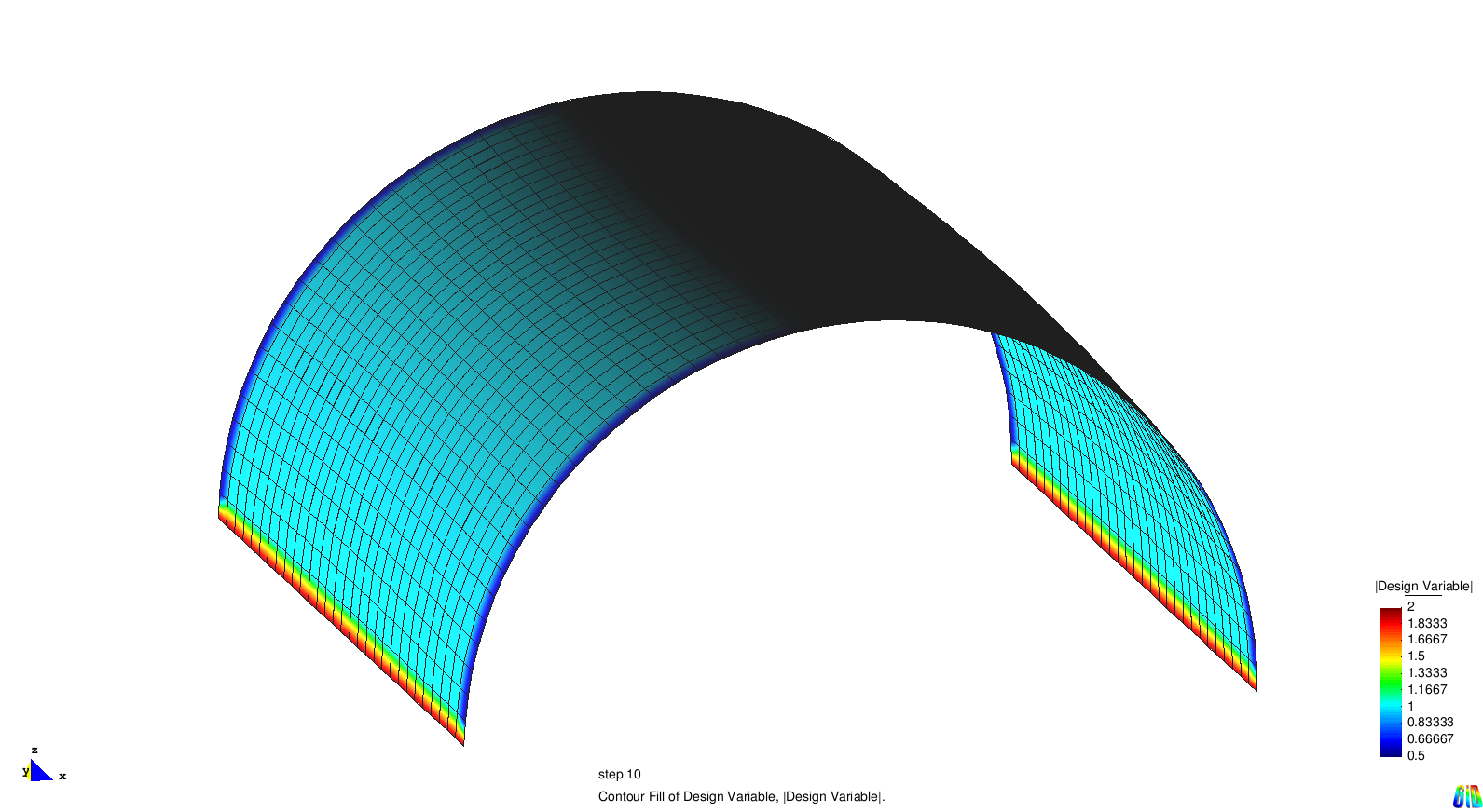
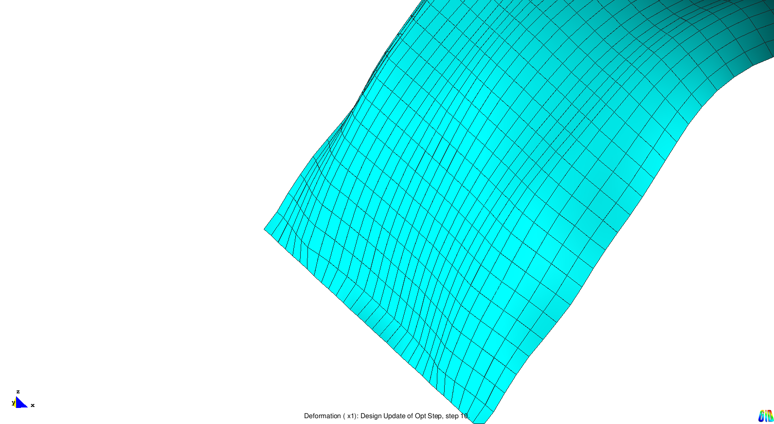
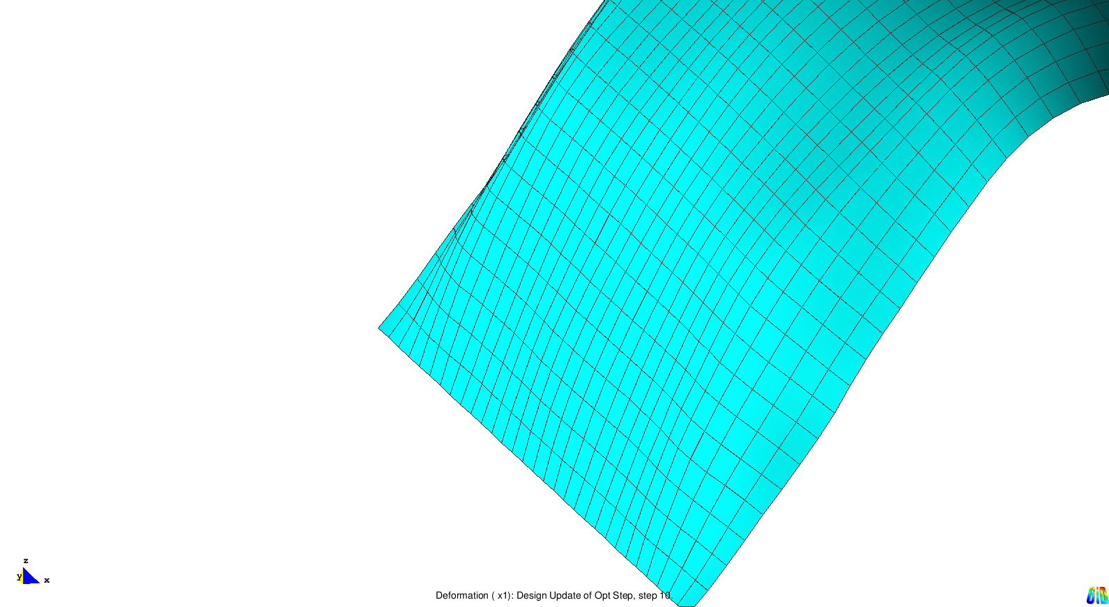
The following example illustrates this topic. We concider a tunnel shell, where the complete structure expect the supports (marked red) is defined to be design space. The first optimization result does not take into account design space bounds and shows a sharp kink towards the supports. In contrast the second picture shows the similar result using the supports as design space bounds and the kink does not appear.
Attention: The parameter BOUNDARY_RADIUS is equipted with a default parameter. To turn off boundary weighting you have to take out the DESIGN_SPACE_BOUNDS of the OPT-CTR.
|
|
|
| Initial geometry with supported nodes (red) | Optimization result without boundary smoothing function | Optimization result using a boundary smoothing function |
Dynamic filter radius control
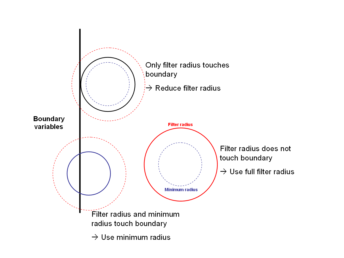
In some cases it might happen that special design variables (e.g. at the edge of a shell) deliver disturbed gardients. To avoid this edge disturbances to be carried far into the design space a dynamic filter radius control can be applied. To this purpose the corresponding edge variables have to be marked as boundary variables (BOUNDVAR=1 in the OPT-VAR block) and the MINIMUM_RADIUS needs to be defined. Now each design variable will automatically choose an individual filter radius depending on its distance to the closest BOUNDVAR variable, the RADIUS and the MINIMUM_RADIUS:
- if RADIUS > distance to closest BOUNDVAR : choose RADIUS as filter radius
- if RADIUS < distance to closest BOUNDVAR and MINIMUM_RADIUS > distance to closest BOUNDVAR : choose distance to closest BOUNDVAR as filter radius
- if RADIUS < distance to closest BOUNDVAR and MINIMUM_RADIUS < distance to closest BOUNDVAR : choose MINIMUM_RADIUS as filter radius
The following picture shows the three possibilities.
Consideration of block interactions
This functionality allows the user to control the filtering by seperating the design variable blocks. Is CONCIDER_BLOCK_INTERACTION set to zero, a design variable only conciders other design variables out of the same OPT-VAR block. If the input flag is set to one, all design variables in the filter radius are taken into account, regardless their block ID.
References
| Whos here now: Members 0 Guests 0 Bots & Crawlers 1 |

