Users:General FEM Analysis/Analyses Reference/Static Linear
Contents |
General Description
The linear static analysis is applied to analyze displacements, strains or stresses of structures. This analysis is valid for linear static mechanical problems without any nonlinearity (geometrically nonlinear, contact, material nonlinear, ...). Static nonlinear problems can be solved by the static nonlinear analysis whereas transient problems are solved by dynamic analysis methods.
The static linear analysis formulates structural equilibrium on the initial configuration without consideration of deformations. Hence, it is only valid for problems showing small displacements.
Structure of Equation System
The linear static analysis solves the problem
K*U=F,
with the linear stiffness matrix K, the unknown displacement fields U and the right hand side vectors F. This system of equations is solved for the unknown displacements by a linear solver. In general, linear solvers may be separated in iterative and direct solvers. Direct solvers transform the stiffness matrix K into an upper diagonal matrix. The displacement field follow by a back substitution with the respective right hand side vector. This back substitution requires only small numerical effort which makes direct solvers very attractive if a couple of displacement fields have to be computed.
Input Parameters
Parameter Description
| Compulsory Parameters | ||
| Parameter | Values, Default(*) | Description |
|---|---|---|
| SOLVER | PC-SOLVER int | Linking to a linear solver (direct or iterative) |
| OUTPUT | PC-OUT int | Linking to output objects (specifies the type of output format, e.g. GiD) |
| COMPCASE | LD-COM int | Linking to computation case objects which specify the boundary conditions (loading and supports) |
| DOMAIN | EL-DOMAIN int | Linking to the domain the analysis should work on |
| Optional Parameters | ||
| ONLY_IBRA_PRE | int | Get integration domain in JSON format for Isogeometric B-Rep Analysis (IBRA) (1 = true, 0 = false) |
| SIMULTANEOUS_EIGENVALUE_ANALYSIS | int | Simultaneous eigenvalue analysis (1 = true, 0 = false) |
| EIGEN_SOLVER | PC-SOLVER int | Linking to a eigenvalue solver |
| NUM_EIGEN_MODES | int | Number of eigenmodes |
| BENCHMARK_ELEMENTS | int | Ids of Design elements |
| BENCHMARK_ELEMENTS_U | float | Position u of the benchmark points in the parameter space. If the number of members equals the number of the ids of the design element, only one point per element is printed. If not, all positions for every element is printed |
| BENCHMARK_ELEMENTS_V | float | Position v of the benchmark points in the parameter space |
| BENCHMARK_ELEMENTS_W | float | Position w of the benchmark points in the parameter space |
| BENCHMARK_DISP | int | if displacement at benchmark point should be printed (1 = true, 0 = false) |
| BENCHMARK_STRESS | int | if stresses at benchmark point should be printed (1 = true, 0 = false) |
| BENCHMARK_OUTPUT_NAME | string | names of files for each benchmark point (default = benchmark_point). If number of output names and design element ids matches, every element is only printed in the respective benchmark output file. For several names write name1,name2,... without spaces |
Example of a Complete Input Block
PC-ANALYSIS 1: STA_GEO_LIN
SOLVER = PC-SOLVER 5
OUTPUT = PC-OUT 1
COMPCASE = LD-COM 1,2,3
DOMAIN = EL-DOMAIN 1
Examples
A Full Example: Bending of a cantilever discretized with shell elements
The following example describes a simple cantilever problem discretized by SHELL8-elements. The respective input file can be found at
- ..\examples\benchmark_examples\elements\shell8_quad_lin_canti_I\shell8_canti_2x20_elem_load.dat
The problem computes three computation cases (dead load, snow load and pressure load). The boundary conditions are visualized by the figure below.
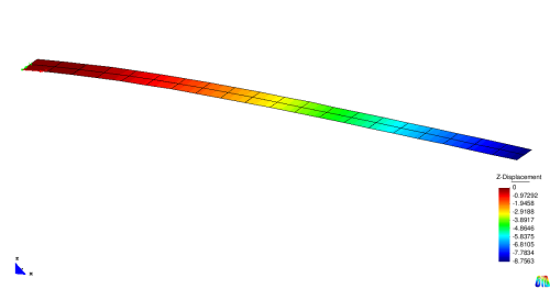
The basic goal of each linear static analysis is the computation of the displacement field. For load case 1 this result is depicted in the figure below, whereas the deformation in z-direction is additionally visualized by the color plot.
It can be seen that the support region does not show any deformation whereas the tip region deforms by a value of 8.76.
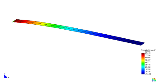
Often the stress distribution is visualized by color plots. Shell structures require the specification of the layer on which the stresses are computed. The picture below shows the first principle stress on the top of the cantilever.
It can be seen that the stresses show maximum values at the support region of the cantilever. At the tip they are nearly zero. In contrast to analytical results the stresses are not exactly zero in numerical models. The reason is the stress computation at the Gauss points. These points are situated inside the elements and not exactly at the tip of the cantilever.
Benchmark examples
- Cantilever under different surface loads, discretized SHELL8-elements ..\examples\benchmark_examples\elements\shell8_quad_lin_canti_I\shell8_canti_2x20_elem_load.dat
- Truss under tension discretized by SOLIDHEXA1-elements: ..\examples\benchmark_examples\analyses\stalin_cantilever_hexa_I\cbm_biegebalken.txt
| Whos here now: Members 0 Guests 0 Bots & Crawlers 1 |


