Users:General FEM Analysis/Analyses Reference/Cutting Pattern

From Carat++ Public Wiki

(Difference between revisions)

Revision as of 16:13, 29 November 2016

General Description

Cutting pattern generation determines a plane and (optimally) stress-free geometry which can be reassembled to build a membrane with a certain prestress and shape (as it was determined in Formfinding).

Structure of Equation System

A nonlinear problem is formulated by the equation r = f_int(u) where r specifies the residual vector and f_int defines the internal forces respectively. In general, the internal forces depend on the actual displacement field u. Thus, the equation is nonlinear with respect to the a priori unknown equilibrium displacements.

At the equilibrium point the residual vector is equal to zero. The above specified nonlinear problem is linearized for the actual displacement state and solved e.g. by a Newton-Raphson scheme where the residual vector is used to compute incremental displacements by K_t u_inc = r.

Input Parameters

Parameter Description

Parameter	Values, Default(*)	Description
Compulsory Parameters
PC-ANALYSIS	int : STA_GEO_NONLIN	Keyword of nonlinear analysis with analysis ID
PATHCONTROL	FORCE or ARCLENGTH or DISPLACEMENT	Definition of path control method. (DISPLACEMENT is actually not available.)
SOLVER	PC-SOLVER int	Linking to a linear solver (direct or iterative)
OUTPUT	PC-OUT int	Linking to output objects (specifies the type of output format, e.g. GiD)
COMPCASE	LD-COM int	Linking to computation case object which specify the boundary conditions (loading and supports). Only a single computation case is allowed.
DOMAIN	EL-DOMAIN int	Linking to the domain the analysis should work on
NUM_STEP	int	Number of time steps that have to be calculated
MAX_ITER_EQUILIBRIUM	int	Maximum number of equilibrium iterations that are allowed.
EQUILIBRIUM_ACCURACY	float	Equilibrium accuracy that has to be reached for convergence. The convergence is checked with the L2 norm of the incremental displacements.
CURVE	LD-CURVE int	Linking to the load curve.
Optional Parameters
TRACED_NODE	int	Node ID of traced node. Used for screen and log file output.
TRACED_NODAL_DOF	dof type	DOF type of node TRACED_NODE that has to be traced (DISP_X, DISP_Y, DISP_Z, ...).
STEP_LENGTH_CONTROL	FIXED or CRISFIELD_RAMM	Type of step length control algorithm (for ARCLENGTH method). FIXED specifies a constant step size where the desired step size is defined by the parameter STEP_LENGTH_CONTROL_REALS. CRISFIELD_RAMM specifies an adaptive method according to Crisfield and Ramm, c.f. ^[1]. In this case the parameter STEP_LENGTH_CONTROL_INTS = int specifies the number of restarts that are allowed. The other necessary parameters are specified by STEP_LENGTH_CONTROL_REALS. See the example below.
STEP_LENGTH_CONTROL_REALS	float, float, ...	respective number of floats for step length control algorithm
STEP_LENGTH_CONTROL_INTS	int, int, ...	respective number of integers for step length control algorithm
SIMULTANEOUS_EIGENVALUE_ANALYSIS	1 or 0	flag to specify if a simultaneous eigenvalue analysis should be performed, 0 - no eigenvalue analysis, 1 - perform eigenvalue analysis. This flag requires definition of parameter EIGEN_SOLVER.
EIGEN_SOLVER	PC-SOLVER int	Linking to an eigenvalue solver
IMPERFECTION_MODES	int, int, int, ...	specifies which eigen modes should be summarized to the imperfection mode. Computation of imperfect design requires definition of parameter EIGEN_SOLVER.
IMPERFECTION_SIZE	float	specifies the size of the imperfection mode.

Example of a Complete Input Block

PC-ANALYSIS 1: STA_GEO_NONLIN
  PATHCONTROL = ARCLENGTH ! or DISPLACEMENT or ARCLENGTH
  SOLVER = PC-SOLVER 1
  OUTPUT = PC-OUT 1
  COMPCASE = LD-COM 1
  DOMAIN = EL-DOMAIN 1
  NUM_STEP = 30
  MAX_ITER_EQUILIBRIUM = 100
  EQUILIBRIUM_ACCURACY = 1e-10
  CURVE=LD-CURVE 1
  TRACED_NODE=2
  TRACED_NODAL_DOF=DISP_Y 
  ! Example: fixed step length of 0.05
    STEP_LENGTH_CONTROL = FIXED
    STEP_LENGTH_CONTROL_REALS = 0.05         ! constant step length of 0.05
  ! Example adaptive step length according to Crisfield and Ramm
    STEP_LENGTH_CONTROL = CRISFIELD_RAMM
    STEP_LENGTH_CONTROL_REALS = 0.1, 1.0     ! initial step length = 0.1, exponent p = 1.0
    STEP_LENGTH_CONTROL_INTS = 5             ! 5 equilibrium iterations per step are desired
  ! Example: no simultaneous eigenvalue analysis
    SIMULTANEOUS_EIGENVALUE_ANALYSIS = 0 
  ! Example: simultaneous eigenvalue analysis
    SIMULTANEOUS_EIGENVALUE_ANALYSIS = 1
    EIGEN_SOLVER = PC-SOLVER 2
  ! Example: use imperfect design with modes 1, 2, 4, and 6
    IMPERFECTION_MODES = 1, 2, 4, 6
    IMPERFECTION_SIZE = 0.015                ! maximum size of imperfection mode equals 0.015
    EIGEN_SOLVER = PC-SOLVER 2

Example

The following simple example shows a geometrically nonlinear analysis of a 2bar truss system using the arclength method. It uses a fixed step size for computation. The respective input file can be found in the SVN repository under

carat20/examples/benchmark_examples/analyses/stanln_2bartruss_arclength_l/2bartruss_arclength_fixed.txt

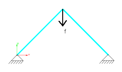
The problem computes a snap through problem. The boundary conditions are visualized by the figure below.

Simple 2bar truss structure discretized with truss elements

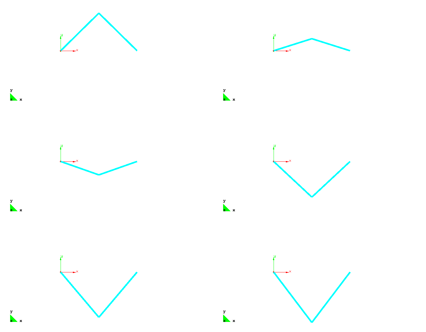
The load f is increased by the arclength method such that the displacements depicted in the figure below occur.

Truss snap through

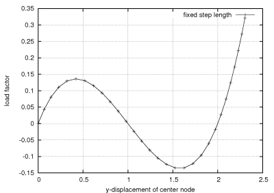
The figure below shows the load displacement path of the y-displacement of the center node. The well known snap through behavior is clearly visible. For a load factor of approx. 0.14 the structure shows instability. In the following the arclength control reduces the load factor until -0.14 to compute equilibrium states. Obviously these states can be only be computed by arclength or displacement control. After a complete snap through the load can be increased further. Now the complete structure works in tension which does not yield to further instability points.

Load displacement path of 2bar truss

References

↑ Cite error: Invalid <ref> tag; no text was provided for refs named Rei94

Whos here now: Members 0 Guests 0 Bots & Crawlers 1

[Rei94] Cite error: Invalid <ref> tag; no text was provided for refs named Rei94

[1]

@@ Line 3: / Line 3: @@
 == General Description ==
-The static nonlinear analysis is applied to analyze displacements, strains or stresses of nonlinear structures. There exists several sources of nonlinearities like nonlinear kinematics, nonlinear material behavior or contact scenarios.
+Cutting pattern generation determines a plane and (optimally) stress-free geometry which can be reassembled to build a membrane with a certain prestress and shape (as it was determined in Formfinding).
-The static nonlinear analysis formulates structural equilibrium on the actual configuration under consideration of the actual system response.
 === Structure of Equation System ===
-A nonlinear problem is formulated by the equation '''r''' = '''f'''_int('''u''') - λ * '''f'''_ext('''u''') where '''r''' specifies the residual vector and '''f'''_int and '''f'''_ext define the internal and external forces respectively. In general, the internal forces as well as the external forces depend on the actual displacement field '''u'''. Thus, the equation is nonlinear with respect to the a priori unknown equilibrium displacements. The parameter λ specifies a scaling parameter for the external load. Usually this parameter is controlled by a load curve which specifies λ as a function of the pseudo time t. The slope of this load curve must be small enough such that convergence is possible in each step. Whenever a nonlinear analysis has convergence problems it is appropriate to reduce the slope of this load curve and calculate more time steps.
+A nonlinear problem is formulated by the equation '''r''' = '''f'''_int('''u''') where '''r''' specifies the residual vector and '''f'''_int defines the internal forces respectively. In general, the internal forces depend on the actual displacement field '''u'''. Thus, the equation is nonlinear with respect to the a priori unknown equilibrium displacements.
-At the equilibrium point the internal forces are equal to the external forces and the residual vector is equal to zero. The above specified nonlinear problem is linearized for the actual displacement state and solved by a Newton-Raphson scheme where the residual vector is used to compute incremental displacements by '''K'''_t '''u'''_inc = '''r'''. Here the tangential stiffness matrix is specified by '''K'''_t whereas '''u'''_inc denotes the incremental displacements.
+At the equilibrium point the residual vector is equal to zero. The above specified nonlinear problem is linearized for the actual displacement state and solved e.g. by a Newton-Raphson scheme where the residual vector is used to compute incremental displacements by '''K'''_t '''u'''_inc = '''r'''.
-=== Path Following Methods ===
-The iterative solution of the nonlinear problem requires path following methods. The most simple path following method is a pure '''Load Control'''. Here the parameter ''lambda'' is increased according to the specified load curve. This allows nonlinear analysis for relatively robust nonlinear problems. But as soon as the structure shows instabilities the load control method usually does not not converge anymore. In this case the '''Arc Length''' method can be applied to compute the equilibrium path. This method controls the so called arc length which is defined as a combination from displacement increment and load increment. In general it is also possible to directly control a specified displacement. But actually this path control method is not available in Carat++. More information about path following methods can be found in the thesis of Reiner Reitinger<ref name="Rei94">Reitinger, R.: Stabilität und Optimierung imperfektionsempfindlicher Tragwerke, Dissertation, Bericht Nr. 17, Institut für Baustatik, Universität Stuttgart, 1994</ref> and Amphon Jarusjarungkiat.
-=== Step Length Control ===
-Actually there exist two methods for step length control in Carat++. The most simple method is the fixed step length which computes the whole load displacement path with a constant step length. This procedure is robust but inefficient because a large number of load steps has to be computed. Usually it is more efficient to apply adaptive step length methods. A very robust method was presented by Crisfield and Ramm, c.f. <ref name="Rei94" />. This method specifies the actual step length for the time step ''i'' by the operation ''StepLength_i'' = ''alpha'' * ''StepLength_i-1''. The parameter ''alpha'' is computed by ''(J_d / (J_i-1 * (Nmb_Restarts+1)))^p'' with: ''J_d'' = desired number of equilibrium iterations, ''J_i-1'' = equilibrium iterations of last time step and ''p'' equals the exponent.
-<pre>
-Example:  Actual iteration step:                                   i
-          Number of desired equilibrium iterations:                J_d = 8.
-          Number of equilibrium iterations in the last time step:  J_i-1 = 12.
-          Number of restarts:                                      Nmb_Restarts = 0.
-          Exponent:                                                p=1.0.
-          Step length of last step:                                StepLength_i-1 = 0.2.
-          alpha = ( 8 / (12*(0+1)))^(1.0) = (8 / 12)^(1.0) = 2/3.
-          StepLength_i = 2/3 * 0.2 = 0.1333.
-</pre>
-Thus, if the number of equilibrium iterations is larger than a desired value the step length is decreased for the next time step. If the number of equilibrium iterations is smaller than a desired value the step length is increased for the next time step. The exponent ''p'' can be used to manipulate the update speed. It should be used with care.
-=== Simultaneous Eigenvalue Analysis ===
-Reaching critical points of the load displacement path (limit points, bifurcation points, ...) requires special investigations. A simultaneous eigenvalue analysis solving the problem ('''K'''_t - ''eigenvalue'' * '''I''') '''phi''' = '''0''' allows for approximation of the load factor at the next critical point ''lambda''_k. Whenever a critical point is reached the above equations yields to a zero eigenvalue. Extrapolating the current load factor according to the eigenvalue allows for good approximations of the critical load.
-=== Imperfect Designs ===
-Many structures subjected to large compression loading are sensitive to geometrical imperfections. Unfortunately the shape of the imperfection is a priori unknown but mostly some information about tolerances exist. In the nonlinear analysis the imperfection shapes can be computed as sum of several  normalized eigenmodes. The final imperfection mode is then scaled by the specified tolerance. This operation can be expressed by d'''x'''_imp = tol * (sum_i '''phi'''_i). After computation of the imperfection mode, the geometry of the structure is modified and the nonlinear analysis starts with the imperfect geometry.
 == Input Parameters ==

Users:General FEM Analysis/Analyses Reference/Cutting Pattern

Revision as of 16:13, 29 November 2016

Contents

General Description

Structure of Equation System

Input Parameters

Parameter Description

Example of a Complete Input Block

Example

References

Views

Personal tools

Content for Users

Content for Developers

Search

Toolbox